In this post, I would like to show how convenient Bayesian modeling is for implementing smoothing. Note that this post has been inspired by the course “Bayesian subnational estimation using complex survey data” given by Jon Wakefield and Richard Li available online.
Prevalence over time
Suppose that we are interested in the population’s proportion with a specific characteristic at a given time point (called the prevalence). Further, assume that it would be too costly or too time consuming to survey all individuals in the population of interest at each time point. Hence, only a sample of the population is surveyed over 81 time points to assess the prevalence’s evolution over time.
The figure below shows points reflecting the sampled prevalence over time (using rbinom() function). The sample size is fixed at \(n=100\) on the left, and \(n=1,000\) on the right. The dashed line represents the true population’s prevalence characterized by an exponential decay as time progresses.
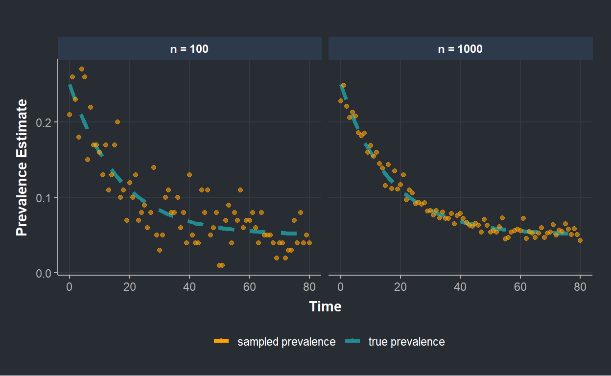
The sample size has a big impact on the precision we have about the prevalence. This is clear from the figure: when \(n=100\), points are much more scattered around the true prevalence than when \(n=1000\). In real life, constraints during the surveying process (time, budget,…) limit the sample size. Thus, we usually end up with prevalence estimates that might be varying over time, just due to the sampling variation (high point to point variation on the left figure). In this context, smoothing/penalization helps in estimating a quantity over time, when we expect that the true underlying prevalence in a population exhibits some degree of smoothness.
Bayesian formula and smoothing
The Bayes formula can be expressed as follows
\[p(\theta|y) \propto L(\theta|y) \times \pi(\theta)\] where we have from left to right, the posterior distribution, the likelihood and the prior distribution. The likelihood describes the distribution of the data, depending on unknown parameters \(\theta\) (see this post). The prior distribution expresses beliefs about \(\theta\) and these beliefs can be expressed in such a way that they provide a mechanism by which smoothing can be imposed.
Modelling the prevalence
In our example, the likelihood should describe the distribution of a prevalence. It is common to model such type of variable with a logistic regression since the outcome variable is binary (an individual has a characteristic or not). This assumption leads to model the logit of \(p\) -where \(p\) is the prevalence we want to estimate- with a linear equation. Let’s write down what we assumed so far
\[ \begin{align} & y_t|p_t \sim Binomial(n, p_t) \\ & log(\frac{p_t}{1-p_t}) = a + \phi_t \end{align} \]
where \(y_t\) is the number of individuals with the characteristic at time \(t\) out of \(n=100\) sampled individuals (\(n\) fixed over time), \(p_t\) is the prevalence we want to estimate, \(a\) consists of an intercept and \(\phi_t\) is a parameter that changes over time. Here comes the prior distribution as a mechanism to impose smoothing: we will assume that \(\phi_t\) is distributed as a random walk of order one. This assumption encourages \(\phi_t\) at \(t\) to be similar to its neighbors. The prior is expressed as
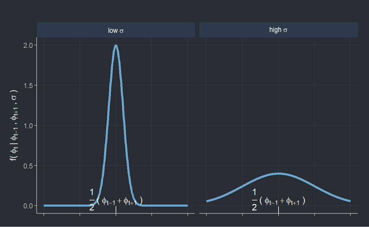
\[ \begin{align} \pi(\phi) & \sim RW1 \\ \Leftrightarrow \phi_t|\phi_{t-1}, \phi_{t+1}, \sigma^2 & \sim \mathcal{N}(\frac{1}{2}(\phi_{t-1} + \phi_{t+1}), \frac{\sigma^2}{2}). \end{align} \]
According to the selected prior distribution, values of \(\phi_t\) close to \(\frac{1}{2}(\phi_{t-1} + \phi_{t+1})\) are favored. It is clear from that distribution that \(\sigma\) can be seen as a smoothing parameter since it defines the spread around \(\frac{1}{2}(\phi_{t-1} + \phi_{t+1})\), which is the middle point between \(\phi_t\)’s two neighbors. The figue below makes it clear that small (large) value of \(\sigma\) enforces strong (weak) smoothing on \(\phi_t\).
Let’s now estimate this model on the sampled proportions using STAN
# STAN code
data {
  int<lower=0> T; // nber of time points
  int<lower=0> n[T]; // sample size (fixed at 100)
  int y[T]; // individual with disease
}
parameters {
  real a;
  vector[T] phi;
  real<lower=0> sigma;
}
transformed parameters {
  vector[T] eta;

  eta = a + phi;
}
model {
  // Likelihood
  y ~ binomial_logit(n, eta);

  // Priors
  a ~ normal(0, 10);

  phi[1] ~ normal(0, sigma); // Random walk 1 for phi
  phi[2:T] ~ normal(phi[1:(T-1)], sigma); // Random walk 1 for phi
  sigma ~ normal(0.5, 0.05);
}
generated quantities {
    vector[T] p_hat = 1 ./ (1+exp(-eta)); // estimated prevalence
}
In the figure below we show the estimated posterior prevalence (with 95% credible interval) where we imposed different priors on \(\sigma\). On the left, we assumed that \(\sigma \sim \mathcal{N}^+(0.5,0.05)\) while on the right, we imposed more smoothing by setting \(\sigma \sim \mathcal{N}^+(0,0.05)\).
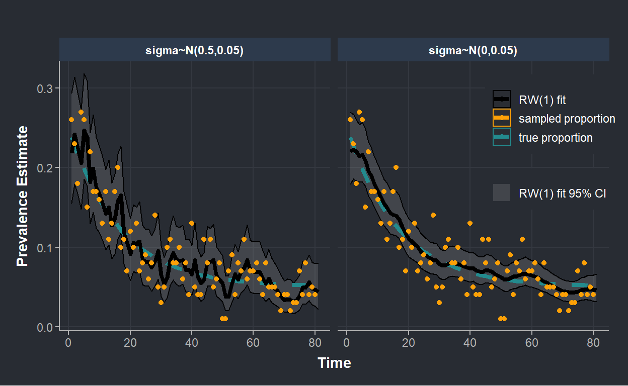
The figure clearly shows that prior distribution can be used to increase smoothing of our estimated posterior prevalence. In fact, the right side of the figure, where we assumed that \(\sigma\)’s distribution is centered on 0, shows much less wiggle than on the left.
Summary
In Bayesian statistics, the posterior distribution of the parameters of interest is proportional to the product of the likelihood and the prior. This post shows that the prior can be used as a mechanism to impose smoothing on the estimated quantity. This makes it straightforward to smooth estimates in a Bayesian estimation framework.